Heat energy plays an essential role in numerous engineering applications, from thermal management in electronic devices to the design of efficient energy systems. Understanding and predicting the movement of thermal energy from regions of high temperature to low temperature within a system is essential for optimizing performance and ensuring safety.

Traditional thermal system designs involve educated guesswork, followed by prototyping and testing, all of which are costly and time-consuming. Today, engineers often rely on mathematical models to analyze and predict heat transfer phenomena. They start by developing equations that describe this process before using a numerical technique to solve the equations.

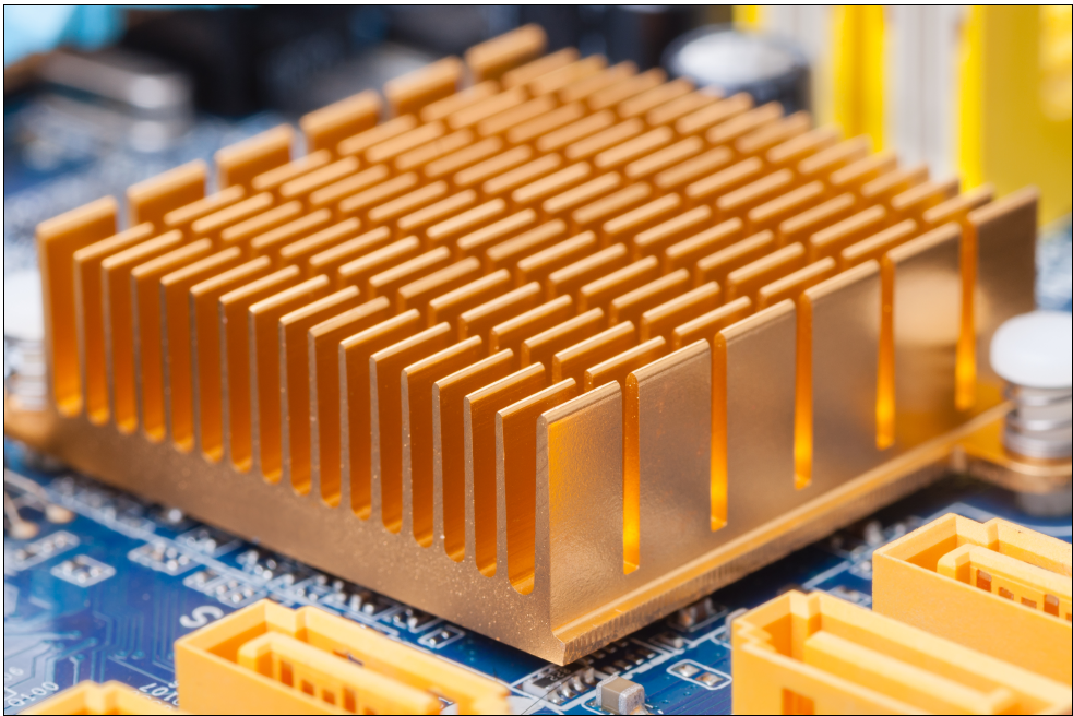Figure 1: Heat energy plays an essential role in numerous engineering applications, from thermal management in electronic devices to the design of efficient energy systems. Source: troninphoto/Adobe Stock

An example of such a numerical technique is the Finite Difference Method (FDM), which can solve partial differential equations representing steady-state heat distribution. But before delving into the basics of the FDM, it is important to present one of the most common and basic equations representing heat transfer.

The basic 2D heat transfer equation

The Laplace equation is a fundamental equation that describes steady-state heat distribution in a medium without any heat source. In its 2D form, this equation is expressed as follows:

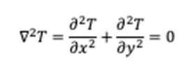Eq1

Where:

T represents the temperature distribution

Eq2 represents the Laplacian operator

The FDM in heat transfer

The FDM is one of the numerical methods often used to solve the Laplace equation. The method starts by discretizing the continuous physical domain into a discrete finite difference grid. Next, the individual exact partial derivatives in the partial differential equation are approximated using finite difference approximations. The finite difference approximations are then substituted into the partial differential equations to obtain algebraic equations at each grid point, which can then be solved for the temperature.

Look at it this way. Suppose there is a need to determine the steady-state temperature distribution in a 2D square plate shown in Figure 2. The boundary conditions of this domain show that the temperature across the top edge of the plate is at 100° C, while the other three edges of the domain are fixed at 30° C.

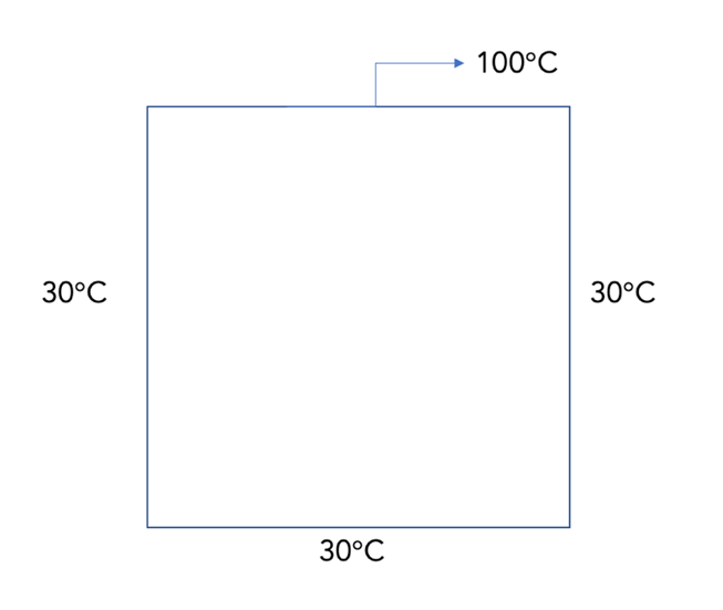Figure 2: 2D plate showing boundary conditions Source: Temitayo Oketola

The FDM requires that this 2D domain is covered by two-dimensional grid lines, called the finite difference grid (see Figure 3). The intersections of these lines are called the grid points, at which the temperature solutions would be obtained. For the present scenario, let’s consider a situation where the grid lines have uniform spacings Eq2 x and Eq2 y, respectively, as shown in Figure 3. The subscripts i and j denote the grid points in the x and y spatial directions, respectively. Therefore, T_ij would represent the approximation of the temperature solution at the grid point located at the ith position along the x-direction and the jth position along the y-direction.

Figure 3: Solution domain covered by two-dimensional gridlines to form grid points where the solution would be obtained Source: Original image from Wonjun1998/CC/SA [4.0].

Next, the partial derivates in the partial differential equation are replaced by centered-space finite difference approximations at each grid point to form a set of algebraic equations. For instance, at any grid point i,j, the finite difference approximation yields:

This simplifies to:

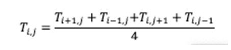
Looking at this equation, it is obvious that the temperature solution at any grid point is the arithmetic average of the solutions at the four neighboring grid points. Therefore, this procedure is repeated for every internal grid point in the domain to form a set of algebraic equations.

Solving the algebraic equations

The algebraic equations are then solved using either a direct method (like the Gauss elimination method) or an iterative method (such as the Jacobi method or the successive over-relaxation method). In this particular scenario, the Jacobi method was used to solve the system of equations.

The Jacobi method is typically used for solving a system of linear equations that is diagonally dominant. The numerical process starts by assuming a guess value (this is what is called the initialization phase). Next, the equations are solved, and the solution is iteratively updated using values from the previous iteration. For instance, in the case of the 2D Laplace equation, the idea can be understood as updating the temperature at each grid point based on the average temperature of its neighboring points. This iterative process is repeated until the error (or difference between the previous and new temperature values) at the grid points is small. At this point, the solution is said to have converged.

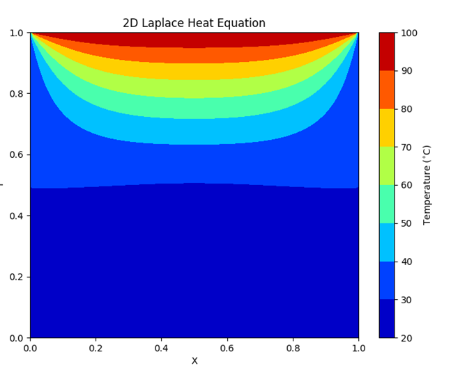
Due to the complexity of the iterative process, engineers typically rely on programming languages to solve these problems. In this particular scenario, a Python code has been developed to solve the 2D Laplace equation for a plate with a dimension of 1 cm by 1 cm, with boundary conditions similar to those specified in Figure 2. Figure 4 shows the result of this iterative process.

Eq7

Conclusion

While this article presents the basics of numerical methods for solving the 2D heat transfer equation, there are several other factors to consider when solving engineering problems using numerical methods. For instance, engineers also have to consider numerical schemes’ consistency, stability and convergence. Moreover, there are several other iterative methods for solving systems of linear equations, and the right method depends on several factors, such as the characteristics of the problem and the properties of the equation.

Learn more about numerical methods by reading engineering texts such as Advanced Engineering Mathematics: A Computer Approach.