Standard inventory models struggle to capture irregular disruptions, inconsistent supplier yields and fluctuating lead times. These factors introduce uncertainty that fixed-parameter approaches cannot represent well, making average-case assumptions unreliable for actual operations. Consequently, planning has shifted toward simulation and stochastic optimization, where inventory policies are tested against delivery failures, delays and variability to account for a wide range of potential scenarios.

This transition moves inventory planning away from static safety stock rules toward more flexible policy structures that remain stable under changing conditions. This methodology involves combining simulation for risk evaluation with optimization for parameter tuning while incorporating operational constraints to keep results implementable. The goal is to maintain balance between service levels, inventory cost and system stability as supply conditions evolve.

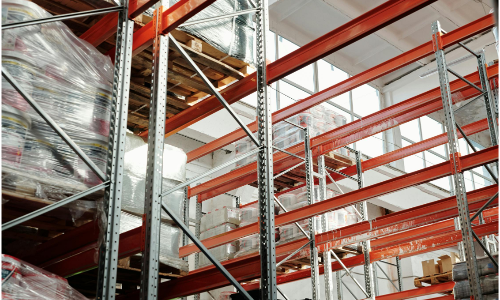Stacked pallets and metal racking in a warehouse. Source: Tiger Lily/Pexels

Computational planning methods

Simulation based approaches typically serve as an evaluation layer. In this framework, a candidate inventory policy defined by reorder points, order quantities and sourcing rules undergoes testing against various disruption scenarios. These scenarios capture variability in lead times and fulfillment. This allows planners to observe how policies perform under stress instead of focusing on expected conditions alone. Optimization is then applied around this layer to refine policy parameters.

In simpler implementations, this involves direct search methods that iteratively adjust reorder thresholds and allocation rules. More structured approaches use stochastic integer programming to incorporate operational constraints such as supplier capacity, budget limits and minimum order quantities. In some cases, risk measures such as conditional value at risk (CVaR) are included to limit expected losses under worst case disruption scenarios.

Two stage approaches are common. An initial simulation phase identifies feasible operating regions and filters out unstable policies. A second stage then refines parameters within those regions using optimization. This separation reduces computational cost and avoids sensitivity to poorly chosen starting conditions.

Model fidelity depends on data quality and update frequency. High resolution models capture short term variability in supplier performance but require frequent recalibration. Lower resolution models are more stable but may smooth over disruption effects that materially impact operations. The appropriate level of detail depends on how quickly supply conditions change relative to the planning cycle.

In practice, fully automated optimization is limited by the need for interpretability and control. Planners define bounds, constraints and acceptable behaviors while the model adjusts parameters within those limits. This keeps policies aligned with operational requirements and reduces the risk of unstable or impractical outputs.

Risk mitigation and control strategies

Once supply variability is modeled, the focus shifts to how inventory policies respond in operation. This requires coordinated adjustments to sourcing, reorder logic and buffer allocation as opposed to treating each in isolation. Multi-sourcing introduces redundancy but also increases variability in lead times and lot sizes. As a result, volume is typically weighted toward more reliable suppliers while secondary sources absorb disruptions. The result is a staggered allocation structure that balances resilience against coordination complexity.

Reorder logic also needs to adapt as fixed thresholds break down under fluctuating yields and delivery timing. Stochastic yield introduces a specific category of risk where the quantity delivered deviates from the quantity ordered. Unlike lead time variation, which affects timing, yield uncertainty creates immediate physical shortages that static safety stock often fails to cover. Policies move away from static reorder points to adjust triggers based on observed supplier performance, treating fulfillment as a probability distribution. This process incorporates recent delays and fulfillment reliability into ordering decisions, scaling order quantities to compensate for expected under-delivery.

Buffering follows the same shift toward selectivity. Inventory is concentrated on components with high disruption impact or long recovery times. This creates an asymmetric structure where a small subset of items carries most of the protective inventory to avoid increasing safety stock uniformly. These decisions are tightly linked. Greater supplier diversification can reduce the need for large buffers. Conversely, more volatile sources may require both higher safety stock and tighter reorder control. The objective is to control how variability moves through the system. When sourcing, timing and inventory are managed as a single structure, disruptions can be absorbed locally to prevent them from compounding across the supply chain.

Performance validation and system tradeoffs

Evaluating an inventory policy under variable supply conditions requires testing it across a range of disruption scenarios to avoid relying on average-case metrics. Performance is typically measured through service level, backorder frequency and recovery time, though these metrics only become meaningful when viewed under variation. Service level targets introduce the most direct tradeoff because the inventory required to support them increases disproportionately under high supply variability. This pushes decisions toward item-specific targets where the cost of additional inventory is weighed against the operational impact of stockouts.

Results are highly sensitive to input assumptions. Policies that perform well under a specific set of lead times or yield conditions can degrade quickly as those inputs shift. Validation focuses on how performance changes as parameters move away from expected values, particularly when disruptions are correlated across multiple suppliers. Update frequency adds another layer to this tradeoff. Frequent updates help track changes in supplier reliability but increase the risk of reacting to short-term noise. Additionally, less frequent updates improve stability at the cost of slower response.

The goal is to identify policies that maintain acceptable performance across these variations to avoid optimizing for a single scenario. Operational reality leads to solutions that are slightly less efficient under ideal conditions but far more stable when supply conditions deviate from plan. Prioritizing consistency over peak efficiency allows operations to remain controlled despite ongoing variability in the supply base.

Toward resilient inventory systems

Inventory system effectiveness depends on planning logic remaining aligned with shifting supply conditions. Success requires a tight link between policy structure and data updates, ensuring supplier performance feeds directly into decision rules. Continuous capture of lead time variability and fulfillment reliability is essential. Without this feedback loop, policies lose effectiveness as conditions change.

Responsiveness is shaped by update frequency and data quality. While faster updates track supplier behavior, they increase sensitivity to short-term noise. Slower updates provide stability but delay responses. This dynamic results in bounded automation where models adjust policies within limits while planners control constraints like order sizes and supplier allocation.

Resilience relies on consistently absorbing disruptions as an alternative to predicting them. Systems maintain stable service levels and predictable recovery when supply conditions move away from plan. The focus shifts toward building structures that dampen variability to avoid reacting to it. Coordinated sourcing, timing and inventory decisions keep disruptions contained.